传统的线性模型难以解决多变量或多输入问题,而神经网络如LSTM则擅长于处理多个变量的问题,该特性使其有助于解决时间序列预测问题。
在接下来的这篇博客中,你将学会如何利用深度学习库Keras搭建LSTM模型来处理多个变量的时间序列预测问题。
经过这个博客你会掌握:
1. 如何将原始数据转化为适合处理时序预测问题的数据格式;
2. 如何准备数据并搭建LSTM来处理时序预测问题;
3. 如何利用模型预测。
目录
1.空气污染预测
在这篇博客中,我们将采用空气质量数据集。数据来源自位于北京的美国大使馆在2010年至2014年共5年间每小时采集的天气及空气污染指数。
数据集包括日期、PM2.5浓度、露点、温度、风向、风速、累积小时雪量和累积小时雨量。原始数据中完整的特征如下:
1.No 行数
2.year 年
3.month 月
4.day 日
5.hour 小时
6.pm2.5 PM2.5浓度
7.DEWP 露点
8.TEMP 温度
9.PRES 大气压
10.cbwd 风向
11.lws 风速
12.ls 累积雪量
13.lr 累积雨量
我们可以利用此数据集搭建预测模型,利用前一个或几个小时的天气条件和污染数据预测下一个(当前)时刻的污染程度。
可以在UCI Machine Learning Repository下载数据集。
Beijing PM2.5 Data Set
2.数据处理
在使用数据之前需要对数据做一些处理,待处理部分数据如下:
No,year,month,day,hour,pm2.5,DEWP,TEMP,PRES,cbwd,Iws,Is,Ir
1,2010,1,1,0,NA,-21,-11,1021,NW,1.79,0,0
2,2010,1,1,1,NA,-21,-12,1020,NW,4.92,0,0
3,2010,1,1,2,NA,-21,-11,1019,NW,6.71,0,0
4,2010,1,1,3,NA,-21,-14,1019,NW,9.84,0,0
5,2010,1,1,4,NA,-20,-12,1018,NW,12.97,0,0
粗略的观察数据集会发现最开始的24小时PM2.5值都是NA,因此需要删除这部分数据,对于其他时刻少量的缺省值利用Pandas中的fillna填充;同时需要整合日期数据,使其作为Pandas中索引(index)。
下面的代码完成了以上的处理过程,同时去掉了原始数据中“No”列,并将列命名为更清晰的名字。
from pandas import read_csv
from datetime import datetime
def parse(x):
return datetime.strptime(x, '%Y %m %d %H')
dataset = read_csv('raw.csv', parse_dates = [['year', 'month', 'day', 'hour']], index_col=0, date_parser=parse)
dataset.drop('No', axis=1, inplace=True)
dataset.columns = ['pollution', 'dew', 'temp', 'press', 'wnd_dir', 'wnd_spd', 'snow', 'rain']
dataset.index.name = 'date'
dataset['pollution'].fillna(0, inplace=True)
dataset = dataset[24:]
print(dataset.head(5))
dataset.to_csv('pollution.csv')
处理后的数据存储在“pollution.csv”文件中,部分如下:
                     pollution  dew  temp   press wnd_dir  wnd_spd  snow  rain
date
2010-01-02 00:00:00      129.0  -16  -4.0  1020.0      SE     1.79     0     0
2010-01-02 01:00:00      148.0  -15  -4.0  1020.0      SE     2.68     0     0
2010-01-02 02:00:00      159.0  -11  -5.0  1021.0      SE     3.57     0     0
2010-01-02 03:00:00      181.0   -7  -5.0  1022.0      SE     5.36     1     0
2010-01-02 04:00:00      138.0   -7  -5.0  1022.0      SE     6.25     2     0
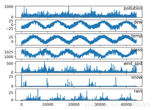
现在的数据格式已经更加适合处理,可以简单的对每列进行绘图。下面的代码加载了“pollution.csv”文件,并对除了类别型特性“风速”的每一列数据分别绘图。
from pandas import read_csv
from matplotlib import pyplot
# load dataset
dataset = read_csv('pollution.csv', header=0, index_col=0)
values = dataset.values
# specify columns to plot
groups = [0, 1, 2, 3, 5, 6, 7]
i = 1
# plot each column
pyplot.figure()
for group in groups:
    pyplot.subplot(len(groups), 1, i)
    pyplot.plot(values[:, group])
    pyplot.title(dataset.columns[group], y=0.5, loc='right')
    i += 1
pyplot.show()
运行上述代码,并对7个变量在5年的范围内绘图。
3.多变量LSTM预测模型
3.1 LSTM数据准备
采用LSTM模型时,第一步需要对数据进行适配处理,其中包括将数据集转化为有监督学习问题和归一化变量(包括输入和输出值),使其能够实现通过前一个时刻(t-1)的污染数据和天气条件预测当前时刻(t)的污染。
以上的处理方式很直接也比较简单,仅仅只是为了抛砖引玉,其他的处理方式也可以探索,比如:
1. 利用过去24小时的污染数据和天气条件预测当前时刻的污染;
2. 预测下一个时刻(t+1)可能的天气条件;
利用上一篇博客中的series_to_supervised()函数将数据集转化为有监督学习问题:How to Convert a Time Series to a Supervised Learning Problem in Python
下面代码中首先加载“pollution.csv”文件,并利用sklearn的预处理模块对类别特征“风向”进行编码,当然也可以对该特征进行one-hot编码。
接着对所有的特征进行归一化处理,然后将数据集转化为有监督学习问题,同时将需要预测的当前时刻(t)的天气条件特征移除,完整代码如下:
def series_to_supervised(data, n_in=1, n_out=1, dropnan=True):
n_vars = 1 if type(data) is list else data.shape[1]
df = DataFrame(data)
cols, names = list(), list()
for i in range(n_in, 0, -1):
cols.append(df.shift(i))
names += [('var%d(t-%d)' % (j+1, i)) for j in range(n_vars)]
for i in range(0, n_out):
cols.append(df.shift(-i))
if i == 0:
names += [('var%d(t)' % (j+1)) for j in range(n_vars)]
else:
names += [('var%d(t+%d)' % (j+1, i)) for j in range(n_vars)]
agg = concat(cols, axis=1)
agg.columns = names
if dropnan:
agg.dropna(inplace=True)
return agg
dataset = read_csv('pollution.csv', header=0, index_col=0)
values = dataset.values
encoder = LabelEncoder()
values[:,4] = encoder.fit_transform(values[:,4])
values = values.astype('float32')
scaler = MinMaxScaler(feature_range=(0, 1))
scaled = scaler.fit_transform(values)
reframed = series_to_supervised(scaled, 1, 1)
reframed.drop(reframed.columns[[9,10,11,12,13,14,15]], axis=1, inplace=True)
print(reframed.head())
运行上述代码,能看到被转化后的数据集,数据集包括8个输入变量(输入特征)和1个输出变量(当前时刻t的空气污染值,标签)
为了使变量名更直观,笔者修改了series_to_supervised()源码。
   pollution(t-1)  dew(t-1)  temp(t-1)  press(t-1)  wnd_dir(t-1)  wnd_spd(t-1)  \
1   0.129779   0.352941   0.245902   0.527273   0.666667   0.002290
2   0.148893   0.367647   0.245902   0.527273   0.666667   0.003811
3   0.159960   0.426471   0.229508   0.545454   0.666667   0.005332
4   0.182093   0.485294   0.229508   0.563637   0.666667   0.008391
5   0.138833   0.485294   0.229508   0.563637   0.666667   0.009912

   snow(t-1)  rain(t-1)   pollution(t)
1   0.000000        0.0  0.148893
2   0.000000        0.0  0.159960
3   0.000000        0.0  0.182093
4   0.037037        0.0  0.138833
5   0.074074        0.0  0.109658
数据集的处理比较简单,还有很多的方式可以尝试,一些可以尝试的方向包括:
1. 对“风向”特征哑编码;
2. 加入季节特征;
3. 时间步长超过1。
其中,上述第三种方式对于处理时间序列问题的LSTM可能是最重要的。
3.2 构造模型
在这一节,我们将构造LSTM模型。
首先,我们需要将处理后的数据集划分为训练集和测试集。为了加速模型的训练,我们仅利用第一年数据进行训练,然后利用剩下的4年进行评估。
下面的代码将数据集进行划分,然后将训练集和测试集划分为输入和输出变量,最终将输入(X)改造为LSTM的输入格式,即[samples,timesteps,features]。
# split into train and test sets
values = reframed.values
n_train_hours = 365 * 24
train = values[:n_train_hours, :]
test = values[n_train_hours:, :]
# split into input and outputs
train_X, train_y = train[:, :-1], train[:, -1]
test_X, test_y = test[:, :-1], test[:, -1]
# reshape input to be 3D [samples, timesteps, features]
train_X = train_X.reshape((train_X.shape[0], 1, train_X.shape[1]))
test_X = test_X.reshape((test_X.shape[0], 1, test_X.shape[1]))
print(train_X.shape, train_y.shape, test_X.shape, test_y.shape)
运行上述代码打印训练集和测试集的输入输出格式,其中9K小时数据作训练集,35K小时数据作测试集。
(8760, 1, 8) (8760,) (35039, 1, 8) (35039,)
现在可以搭建LSTM模型了。
LSTM模型中,隐藏层有50个神经元,输出层1个神经元(回归问题),输入变量是一个时间步(t-1)的特征,损失函数采用Mean Absolute Error(MAE),优化算法采用Adam,模型采用50个epochs并且每个batch的大小为72。
最后,在fit()函数中设置validation_data参数,记录训练集和测试集的损失,并在完成训练和测试后绘制损失图。
# design network
model = Sequential()
model.add(LSTM(50, input_shape=(train_X.shape[1], train_X.shape[2])))
model.add(Dense(1))
model.compile(loss='mae', optimizer='adam')
# fit network
history = model.fit(train_X, train_y, epochs=50, batch_size=72, validation_data=(test_X, test_y), verbose=2, shuffle=False)
# plot history
pyplot.plot(history.history['loss'], label='train')
pyplot.plot(history.history['val_loss'], label='test')
pyplot.legend()
pyplot.show()
3.3 模型评估
接下里我们对模型效果进行评估。
值得注意的是:需要将预测结果和部分测试集数据组合然后进行比例反转(invert the scaling),同时也需要将测试集上的预期值也进行比例转换。
(We combine the forecast with the test dataset and invert the scaling. We also invert scaling on the test dataset with the expected pollution numbers.)
至于在这里为什么进行比例反转,是因为我们将原始数据进行了预处理(连同输出值y),此时的误差损失计算是在处理之后的数据上进行的,为了计算在原始比例上的误差需要将数据进行转化。同时笔者有个小Tips:就是反转时的矩阵大小一定要和原来的大小(shape)完全相同,否则就会报错。
通过以上处理之后,再结合RMSE(均方根误差)计算损失。
yhat = model.predict(test_X)
test_X = test_X.reshape((test_X.shape[0], test_X.shape[2]))
inv_yhat = concatenate((yhat, test_X[:, 1:]), axis=1)
inv_yhat = scaler.inverse_transform(inv_yhat)
inv_yhat = inv_yhat[:,0]
test_y = test_y.reshape((len(test_y), 1))
inv_y = concatenate((test_y, test_X[:, 1:]), axis=1)
inv_y = scaler.inverse_transform(inv_y)
inv_y = inv_y[:,0]
rmse = sqrt(mean_squared_error(inv_y, inv_yhat))
print('Test RMSE: %.3f' % rmse)
整个小项目完整代码如下,注意:下例代码假设你已经正确地完成了数据预处理过程,如将下载的“raw.csv” 数据处理成 “pollution.csv“文件中的数据。
from math import sqrt
from numpy import concatenate
from matplotlib import pyplot
from pandas import read_csv
from pandas import DataFrame
from pandas import concat
from sklearn.preprocessing import MinMaxScaler
from sklearn.preprocessing import LabelEncoder
from sklearn.metrics import mean_squared_error
from keras.models import Sequential
from keras.layers import Dense
from keras.layers import LSTM
def series_to_supervised(data, n_in=1, n_out=1, dropnan=True):
n_vars = 1 if type(data) is list else data.shape[1]
df = DataFrame(data)
cols, names = list(), list()
for i in range(n_in, 0, -1):
cols.append(df.shift(i))
names += [('var%d(t-%d)' % (j+1, i)) for j in range(n_vars)]
for i in range(0, n_out):
cols.append(df.shift(-i))
if i == 0:
names += [('var%d(t)' % (j+1)) for j in range(n_vars)]
else:
names += [('var%d(t+%d)' % (j+1, i)) for j in range(n_vars)]
agg = concat(cols, axis=1)
agg.columns = names
if dropnan:
agg.dropna(inplace=True)
return agg
dataset = read_csv('pollution.csv', header=0, index_col=0)
values = dataset.values
encoder = LabelEncoder()
values[:,4] = encoder.fit_transform(values[:,4])
values = values.astype('float32')
scaler = MinMaxScaler(feature_range=(0, 1))
scaled = scaler.fit_transform(values)
reframed = series_to_supervised(scaled, 1, 1)
reframed.drop(reframed.columns[[9,10,11,12,13,14,15]], axis=1, inplace=True)
print(reframed.head())
values = reframed.values
n_train_hours = 365 * 24
train = values[:n_train_hours, :]
test = values[n_train_hours:, :]
train_X, train_y = train[:, :-1], train[:, -1]
test_X, test_y = test[:, :-1], test[:, -1]
train_X = train_X.reshape((train_X.shape[0], 1, train_X.shape[1]))
test_X = test_X.reshape((test_X.shape[0], 1, test_X.shape[1]))
print(train_X.shape, train_y.shape, test_X.shape, test_y.shape)
model = Sequential()
model.add(LSTM(50, input_shape=(train_X.shape[1], train_X.shape[2])))
model.add(Dense(1))
model.compile(loss='mae', optimizer='adam')
history = model.fit(train_X, train_y, epochs=50, batch_size=72, validation_data=(test_X, test_y), verbose=2, shuffle=False)
pyplot.plot(history.history['loss'], label='train')
pyplot.plot(history.history['val_loss'], label='test')
pyplot.legend()
pyplot.show()
yhat = model.predict(test_X)
test_X = test_X.reshape((test_X.shape[0], test_X.shape[2]))
inv_yhat = concatenate((yhat, test_X[:, 1:]), axis=1)
inv_yhat = scaler.inverse_transform(inv_yhat)
inv_yhat = inv_yhat[:,0]
test_y = test_y.reshape((len(test_y), 1))
inv_y = concatenate((test_y, test_X[:, 1:]), axis=1)
inv_y = scaler.inverse_transform(inv_y)
inv_y = inv_y[:,0]
rmse = sqrt(mean_squared_error(inv_y, inv_yhat))
print('Test RMSE: %.3f' % rmse)
运行以上代码,首先将会绘制训练过程中的训练和测试损失图。
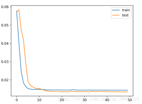
训练中的每个epoch都会记录和绘制训练集和测试集的损失,并在整个训练结束后绘制模型最终的RMSE。
下图中可以看到,整个模型的RMSE达到26.496。
...
Epoch 46/50
0s - loss: 0.0143 - val_loss: 0.0133
Epoch 47/50
0s - loss: 0.0143 - val_loss: 0.0133
Epoch 48/50
0s - loss: 0.0144 - val_loss: 0.0133
Epoch 49/50
0s - loss: 0.0143 - val_loss: 0.0133
Epoch 50/50
0s - loss: 0.0144 - val_loss: 0.0133
Test RMSE: 26.496
4.进一步阅读
如果你想继续深入研究,本节提供更多的阅读资源:
1. Beijing PM2.5 Data Set on the UCI Machine Learning Repository
2. The 5 Step Life-Cycle for Long Short-Term Memory Models in Keras
3. Time Series Forecasting with the Long Short-Term Memory Network in Python
4. Multi-step Time Series Forecasting with Long Short-Term Memory Networks in Python
由于博客中代码展示不太方便,本人已将代码上传至Github中,欢迎指正交流。


 1万+
1万+ 